Survivability in Object Services Architectures

Estimating Service Failure

David L. Wells
David E. Langworthy

Object Services and Consulting, Inc.

In the process of creating and maintaining survivable configurations, the Survivability Service needs to predict the likelihood that, within some time interval, a service will be damaged to an extent that it cannot provide the required level of service. This paper discusses a basic model of how services are provided by resources, how threats against those services are modeled, and how the probability of service failure is computed from the threat model.

1. Introduction

While creating and maintaining survivable configurations, the Survivability Service needs to predict the likelihood that, within some time interval, a service will be damaged to an extent that it cannot provide the required level of service.

This report presents a general model of how services are provided by resources, how threats against those services are modeled, and how the probability of service failure is computed from the threat model. The general model allows substantial flexibility in the details of how resources and threats are modeled; this constitutes and important parameterization of the Survivability Service.

In order for the Survivability Service to function, at least one specialization of the general model must be defined; the model specialization currently used by the Survivability Service is presented. Of course, in order for the Survivability Service to actually function, there must be a concrete realization describing the properties of the particular software system being monitored, specified as defined by the model specialization being used. Such a concrete realization is outside the scope of this report.

In general, the failure computations can be computationally intensive. We present a number of optimizations to reduce the effort required to estimate failure probabilities.

The report conclude with issues related to the general model and our particular specialization.

2. General Model

Estimation of service failure requires a model of resources available within the system, a model of threats to those resources, and calculating techniques to apply the threats to the resources. This section defines the most generalized form of each of these that must be adhered to by any specialization.

The generalized model must be able to express:

independent threats to individual resources,
attacks that affect multiple resources,
multiple attacks against the same resource,
correlated attacks on groups of resources,
variable probabilities of resources being affected by attacks,
ongoing attacks,
variable amounts of damage by attacks,
simple resources that do not depend on other resources,
complex resources that depend on other resources, and
multiple levels of resource quality of service.

Not all of these need be supported by a particular specialization.

2.1. General Resource Model

Resources. Every service is provided by a resource. A resource may be either a base resource or a complex resource. Complex resources use the services provided by other (base or complex) resources; base resources do not. A base resource is affected only by its own failure, while complex resources are affected by the failure of resources upon which they depend. It is typical that services specify only the services upon which they directly rely. However, nested dependencies exist whenever a resource relies upon the services of a complex resource which will itself have dependencies. In this case, a failure of a lower level resource may cause the failure of a higher level service. We define the resource closure of a service in the obvious way. The resource closure may be represented as a directed graph of resource dependencies.

Any cut through the resource closure graph of a service represents a set of resources, either base or complex, on which the service relies. Such a set is called a resource group of the service.

A resource group R is denoted as:

R = {r₁, .., r_n}
where:

There are potentially many (equivalent) resource groups for a given service, depending on where the cut is made. Only one of these contains exclusively base resources.

Consider a simple planning service example. The planning service directly relies upon five resources: its own code, the computer the planning service currently runs on, a map service, a weather service, a network connection to the map service, and a network connection to the weather service. The map and weather services are themselves complex services, while the planning service's code, its computer, and the network connections can be modeled as base resources. The map and weather services, each rely on a host and some software. The planning service does not directly care (or even know) about the resources used by the map and weather services as long as those services continue to perform. However, since a map host failure will cause the map service to fail, which will in turn cause the planning service to fail, these base resources are included in the resource closure of planning service and consequently are of concern to the Survivability Service.

Resource States: Damage causes the state of a resource to change (unless it was already failed). A specialization of the resource model must define the potential states of each resource. More states increases the realism of the model at the cost of increased storage and computational complexity. Natural choices for resource states are:

{Fail, Run} if resources are considered to be either functioning perfectly or not at all (or at least insufficiently well to be useful),
percentage degradations (e.g., lose 20% of capacity) to describe diminished capability to provide QoS for resources whose level of service is easily measured (e.g., CPU cycles), or
QoS states (e.g., High, Low, Failed) for services whose QoS level is not easily measured quantitatively, or where there is a desire to reduce the number of QoS levels to a more manageable number as is done in the QuO system.

Just as individual resources will be in some state, so will resource groups. The state space of a resource group is the cross product of the potential states of the individual resources in the resource group. A state of a resource group is one particular element in this state space. The state space of a resource group grows rapidly with group size and number of states for the individual resources. For this reason, it is important that there be ways to prune portions of the space as irrelevant for common cases. These are discussed below.

The state of a resource group is important because we generally care less about the state of individual resources than we do about the state of configurations of resources. There are three reasons for this:

providing a complex service requires many resources of different kinds,
not all resources in a resource group are necessarily required, and
there is often substantial freedom in the choice of configuration; if one doesn't work, another might.

A resource group will be in exactly one state at any given time. Since a service is itself a resource, it will be in some state as well. There is a mapping from resource group states to service states that indicates the state(s) possible for the service given the states of the resources. Note that this is not strictly a function, since a service might choose to operate in a lower state than is possible given its resources (for example because its client does not currently demand a higher level of service). In general, the service will be attempting to operate in some state, so it will be possible to tell, from the state of its resource group, whether it will be successful.

Probability Distribution of State Spaces: It is common to need to estimate the probability that a service will be able to function in a particular state given its current (or planned future) resource group. This means that it is useful to describe the potential of a resource group for being in any of its possible states. The probability distribution of the state space of a resource group is an assignment of a probability to each potential state. Naturally, the probabilities must be in [0.0 .. 1.0] and must sum to 1.0.

2.2. General Threat Model

Threats: All resources are subject to threats. A threat is the potential for damage to some collection of resources. These resources are said to be vulnerable to that threat and are called that threat's vulnerable resource group. Vulnerable resources can be damaged if the threat manifests itself as an attack. An attack can cause damage to zero or more of the vulnerable resources. Sometimes this damage is correlated (resources are likely to be affected together in the same way) and sometimes it is not. When a resource is damaged, it moves to one of its lower potential states depending on the nature of the threat. Damage to resources changes the state of the resource group.

A threat T is defined as:

T = (R, D(R))
where:

R is the vulnerable resource group
D(R) is a damage effect matrix specifying the probability of transitioning, within some time interval, from any resource group state to any other resource group state because of damage from an attack

Note that D(R) defines the probabilities of transition within some time interval. D(R) can be huge, so for pragmatic purposes, it is important to define a threat model in which relevant parts of D(R) can be computed from a smaller specification. This is discussed below.

Restricting Threats to Resource Groups: Ultimately, we care about the effect of threats on services' resource groups; i.e., being able to compute the probability distribution of the state space for arbitrary resource groups given known threats. It will frequently be the case that the vulnerable resource group for a threat contains resources that are not part of the resource group for a service under investigation and vice versa. While an attack based on the threat may cause resources outside the service resource group to fail, we will generally be unconcerned with this. For this reason, it is useful to be able to restrict a threat to only those elements in the service resource group. A restricted threat is one whose definition has been modified by subsetting the vulnerable resource group and making modifications to D(R) to limit transitions to the subset with the appropriate transition probabilities.

If a resource group V is vulnerable to a threat T, then any subset of V is also vulnerable to T. The implication of this is that the intersection of the vulnerable resource group of a threat and the service resource group of a service is also a vulnerable resource group for the threat. This means that for any threat T with resource group R_T and service S with resource group R_T, it is possible to compute the definition of a restricted threat T' whose vulnerable resource set is this intersection and whose stochastic state transition matrix applies only to the intersection. Resources in the service resource group that are not vulnerable to the threat cannot be affected, but must be considered when defining the damage matrix.

A restriction T' of a threat T to a service S is defined as:

T' = (union(intersect(R_T, R_S), R_S), D(union(intersect(R_T, R_S), R_S))

The computation of D(union(intersect(R_T, R_S), R_S) is dependent upon the form of D(R_T) and D(R_S). The way to compute this for our specialization of the threat model is discussed below .

Threats to Complex Resources: In principle, it would be possible to define threats that applied to entire services. However, this is unsatisfactory for a variety of reasons:

It is far harder to make realistic estimates of the vulnerability of complex things (services) than simple things (base resources). Threats to base resources are generally simpler and more uniform because of the uniformity of base resources. For example, the threat of hardware failure is the same for all identical SPARC stations and all copies of the same code will have the same programming errors. As a result, all functionally similar resources are subject to the same threats. Complex resources, on the other hand, are constructed from simpler resources and they may be constructed in a variety of ways. Two functionally equivalent map servers may utilize very different kinds of base resources and thus be subject the quite different threats.
Many kinds of threats to base resources are already known. For example, analyses of hardware failure rates are common, insurance companies make their living by accurately estimating the likelihood of physical disasters such as fires and floods, and the SEI and others are working on ways to measure software quality. The same is not true for complex services that rely on many resources.
The number of individual services for which threats would have to be individually specified is daunting,
Modeling threats against directly against complex services ignores the fact that services can be reconfigured to use different resources.
Modeling threats against directly against complex services ignores correlation between failures of different services. This is particularly critical when considering relicas, where correlated failures may make a system far less robust than it might appear on the surface, or when two services rely on the use of common base resources.

For this reason, we choose to directly model threats against base resources and aggregate them to determine the threats against more complex resources. Threats to base resources are identified and defined by a human and stored in a database accessible to the Survivability Service. Threats to complex resources are computed from these. Note that if a service is a black box, it can be modeled as a base resource, but then the Survivability Service will have little latitude in helping it survive.

2.3. Computing the Effect of Threats on Services

2.3.1 Overview of the Calculations

Computing the effect of threats on a service proceeds as follows:

The resources used by the service are determined. This will typically require recursively following sequences of single level resource dependencies through intermediate services down to base resources. Base resources must be reached, since it is only for base resources that threats are stored in the concrete threat model. The resource dependencies may be represented as either a directed graph whose intermediate nodes are intermediate level services, or flattened into a state space of base resources.
The states of the resource group that will allow the service to function as desired are determined. This information is used to derive a function that maps the probability distribution of the resource group's state space to a probability that the service continues to perform.
The damage effect matrices of the threats (as restricted to the resource group) are applied to the resource group to determine the probability distribution of the resource group's state space.
The probability of the service being able to perform as desired is computed from the probability distribution of the service resource group's state space using the function derived in step #2.

2.3.2. Computing with a Flattened State Space

The most general form of the computation flattens the resource group to base resources. For even moderate sized resource groups, this computation is intractable, so a number of optimizations are used to manage the computational complexity. However, because it represents the most conceptually clear form of the calculation, it is presented first, followed by the various optimizations.

The resource group is represented by a state space formed as the cross product of all possible states of all base resources in the resource closure. The resource dependency graph can be used to determine which states will allow the service to perform and which will not. States of a resource group that allow a service to function can be framed as a Boolean expression over the resources in the resource group. For each complex resource in the expression, replace it by the Boolean expression describing states of its resource group needed to function. Repeat this until all complex resources are eliminated. The resultant expression can be simplified if desired.

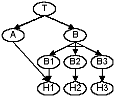
Consider the example below.

In the example we have a high level resource T. T depends on a service A which runs on host H1. In addition, T depends on a replica group B. B depends on three replicas B1, B2, and B3. In the diagram the bar across the links indicates an "or" dependency rather than the standard "and" dependency. B1, B2, and B3 depend on H1, H2, and H3 respectively. Service A runs application code A' and replicas B1, B2, and B3 all run application code B'. The replicas of B are coordinated by code C'. For simplicity, assume that a resource (host or code) either performs or fails.

T performs if A and B both perform. A performs if A' and H1 both perform. B performs if C' and any of B1, B2, or B3 perform. Bi performs if B' performs and Hi performs. Thus, a state in the resource group state space will allow T to perform if it satisfies:

(A' and H1) and (C' and B' and (H1 or H2 or H3))

Naturally, alternate forms of this expression are possible.

The probability distribution of the state space is computed iteratively by applying the damage matrices of the restricted threats. At each iteration, we will have the probability distribution for the state space given threats that have been considered so far. The initial state (actual or believed) is determined directly from the monitors (sensors).

Once the probability distribution of the resource group state space has been computed, the probability that the service will function is a simple matter of summing the probabilities of being in each of the states that satisfy the function computed above.

2.3.3. Generic Optimizations

The procedure outlined above is computationally intensive and creates large closures. Fortunately, in many configurations, it is possible to simplify this process substantially.

Optimizations of the following kinds are possible, depending on the particular model specialization chosen:

reducing the size of the resource group state spaces, which will in turn shrink the size of the matrices for state space probability distributions and damage effects,
specifying threats in such a way that it is possible to compute (rather than specify) the damage effect matrices in most cases; to do this, we differentiate between threats to base resources and threats to complex resources,
pruning techniques to be able to coalesce equivalent states or to avoid computations altogether when their effect is insignificant,
recursive techniques to hide inherited resource dependencies when considering complex services with many levels of dependencies to reduce state space explosion while not losing the effect of threats against possibly shared lower level resources.

The optimizations mentioned above make use of properties of the kinds of configurations maintained by the Survivability Service. Our survivable object abstraction (see our Composition Model and Evolution Model papers) places certain restrictions on the form of resource dependency graphs. At any single level of abstraction, there are three basic resource dependency structures:

all of a collection of potentially diverse resources are required,
at least one of a collection of functionally equivalent replicas are required, and
some quorum q>1 of functionally equivalent replicas are required.

These techniques are applicable to many specializations, but for clarity, we will explain them in the context of our own specialization.

3. A Specialization of the General Model

The general resource model, threat model, and calculations presented above are very powerful. The general model leaves free the choice of possible resource states and the algebra for the damage effect matrix, since this degree of freedom is necessary in order to support different survivability and QoS policies. A specialization must define these. Also to be defined is a concrete representation for resources and threats.

While specializing the general model, it is desirable to keep in mind that the general model is extremely space and computation intensive, so it is important that the specialization be amenable to optimizations that make specification, storage, and computation tractable. This section presents such a model. It satisfies most of the desired properties (reiterated below) provided by the general model and is computationally much more efficient. Desired properties satisfied by the specialization are denoted by a "*".

independent threats to individual resources (*),
attacks that affect multiple resources (*),
multiple attacks against the same resource (*),
correlated attacks on groups of resources (*),
variable probabilities of resources being affected by attacks (*),
ongoing attacks (*),
variable amounts of damage by attacks,
simple resources that do not depend on other resources (*),
complex resources that depend on other resources (*), and
multiple levels of resource quality of service.

3.1. Resource States and Damage Effects

Restricting the resource states that will be modeled is key to making the computation tractable, since if there are m allowable states, a resource group with n elements will have mⁿ states. If an attack can cause any combination of resources to transition to any lower resource states, then for m states and n resources, the damage effect matrix must contain (m*(m+1)/2)ⁿ entries. [Note: proof by induction on m.]

We consider only two possible states for resources: {Failed, Running}. The state space of a resource group is thus (F, R)^*. This also means that the damage effects are limited to {Fail, NotFail}.

3.2. Threats to Base Resources

As noted above, there are several differences between threats to base resources and threats to complex resources that cause us to only directly specify threats to base resources. These same differences allow us to model threats to base resources in a simpler, more compact fashion than is required for threats to arbitrary (potentially complex) resources by the general model. In particular, there is a much simpler, more compact way to specify the potential effect of a threat that eliminates the need to specify a complete damage effect matrix for threats to base resources.

3.2.1 Threat Specifications

Recall that in the general model, a threat T is defined as: T = (R, D(R))
where:

R is the vulnerable resource group
D(R) is a damage effect matrix specifying the probability of transitioning from any resource group state to any other resource group state because of damage from an attack

As seen, D(R) can quickly become huge, so there is an incentive to create a more compact form. Even with the only resource states being {Running, Failed} and the only transitions being {Fail NotFail}, the size of of the damage effect matrix for an n element resource group is 3ⁿ. The matrix can be further reduced in size by observing that Fail(X)=Failed and NotFail(X)=X. Thus, it is sufficient to give the probabilities of failure for all possible combinations of resources in the group. This is 2ⁿ entries (probabilities) for a resource group with n elements.

However, this is still large. We can do better by observing that a resource is only damaged if a threat materializes as an attack and by then assuming that in the event of an attack, all base resources have equal probability of failure. A specification of this type looks like:

_simple-base

R is the vulnerable resource group
P(A) is the probability of an attack materializing in the time period as the result of the threat
P(Fail(r)|A) is the probability that each resource in R fails if an attack occurs

>From this, the stochastic state transition matrix can be computed easily (see below).

This model is realistic for many kinds of threats. The following examples show how different situations can be represented in this model of base threats.

Example #1 - Independent Failures: A and B are hosts in different mobile platforms, The threat is that the platform (and hence the computer) will be destroyed; there is a 0.01 probability of that happening during our interval. The platforms are independent, and equally likely to be destroyed.

T_destroyed = ({A, B}, 1.0, 0.01) Example #2 - Attacks Against Multiple Resources: C and D are hosts that rely on the same power supply. The threat is that the power supply fails; there is a 0.01 probability that is happens during our interval. If this happens, both A and B will fail; if it does not happen, neither will fail as a result of that threat. T_power = ({C, D}, 0.01, 1.0) Example #3 - Correlated Attacks: E and F are programs that are susceptible to a viral attack. There is a 0.04 probability that such an attack will be launched during our interval, and that if it is, there is a 0.25 probability that each of E and F crash. T_virus = ({E, F}, 0.04, 0.25)

3.2.2. Computing the Damage Effect Matrix

The restriction of the damage effect matrix for a threat to a group of base resources is computed as follows. Assume the restricted vulnerable set R has n members. In our model, failures are independent if an attack occurs, so the number of failed resources, m, in the event of an attack is binomially distributed; i.e., p(n, m)= P(Fail(r)|A)^m* (1-P(Fail(r)|A))^n-m . In addition, no resources fail if no attack occurs. So:

P(transition to a state with m>0 failed resources) = P(A) * P(Fail(r)|A)^m* (1-P(Fail(r)|A))^n-m
P(no failures) = (1 - P(A)) + (P(A)*(1-P(Fail(r)|A))ⁿ)

Resources outside the vulnerable resource group cannot be affected by the threat, so the probability of transition to states in which they Fail is zero.

Example #4: T_virus ({E, F, X}, 0.04, 0.25) applies to a service with resource group {E, F, Y}. The restriction of T_virus is:

T_virus' = ({E, F, Y}, 0.04, [(RRR, 0.9825)     // 1 - 0.04 + 0.04*(1-0.25)²
(RRF, 0.0000)     // Y cannot fail
(RFR, 0.0075)     // 0.04 * 0.25¹ * (1-0.25)¹
(RFF, 0.0000)     // Y cannot fail
(FRR, 0.0075)     // 0.04 * 0.25¹ * (1-0.25)¹
(FRF, 0.0000)     // Y cannot fail
(FFR, 0.0025)     // 0.04 * 0.25² * (1-0.25)⁰
(FFF, 0.0000)])   // Y cannot fail

3.2.3. Expressiveness of the Specialization

Examples #1-3 represent, respectively, independent failures, attacks against multiple resources, and correlated attacks. Consider the following table, which shows the probability that particular configurations of AB, CD, and EF are functioning at the end of our interval. An R indicates the resource is running, an F indicates it has failed.

AB	P		CD	P		EF	P
RR RF FR FF	0.9801 0.0099 0.0099 0.0001		RR RF FR FF	0.9900 0.0000 0.0000 0.0100		RR RF FR FF	0.9825 0.0075 0.0075 0.0025

Since we care about which subset(s) of the resource group are likely to end up in, this distinction matters. Since the important subsets are often either the entire resource group (i.e., [RR]) or those with at least one surviving member (i.e., not [FF]), the need to consider correlation is clear. The case where a resource is shared among the resource groups of multiple services is similar.

This specialization accurately captures two critical survivability notions (assuming that failure probabilities are similar):

when all resources in a resource group must survive, it is best to choose resources whose failures are correlated, since this reduces the number of ways in which resources can be compromised
when only some (e.g., replicated) resources in a resource group must survive, it is best to choose those whose threats have as little correlation as possible, since this prevents a small number of attacks from affecting many resources.

Because this specialization divides a threat into a probability that an attack will occur and a probability that a resource is affected if the attack occurs, it is possible to make use of recent history to improve the use of the model. If some resource has been damaged by an attack and the attack is of the sort that can last through multiple time intervals (as most can), then we know that an attack is in progress and therefore P(A)=1. The result is that other resources subject to the threat are more likely to be damaged than they would be if it were not known that the threat had manifested itself as an active attack. This deals nicely with the "burning building problem". While it is generally a good idea to not place critical resources such that they can be damaged by a single fire, it is essential to avoid such configurations the fire is occurring right now. Of course, similar observations apply to other kinds of threats as well, where we might want to avoid over reliance on one platform type to avoid hacker attacks, but the need to do so becomes much more critical when such attacks are known to be occurring.

3.3. Threats to Complex Resources

A complex resource (service) is threatened by the failure of lower level resources upon which it relies. As such, it is threatened by the same threats as these lower level resources. The example below illustrates the straightforward manner of computing how threats to complex resources are determined based on threats to base resources. Optimizations are discussed in the next section.

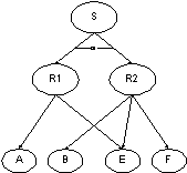
Example #5 - Threats to Complex Resources. A service S requires at least one replica from the set {R1, R2 }. Dependencies of the replicas are:

Threats to these resources are:

T_destroyed = ({A}, 1.0, 0.01)

T_power = ({A, B}, 0.01, 1.0)

T_virus = ({E, F}, 0.04, 0.25)

S performs if it satisfies:

S = R1 or R2 = (A and E) or (B and E and F) = E and (A or (B and F)) The only states for [ABEF] that satisfy this equation are:

The damage effect matrices are shown below. Transitions not shown have P=0. N represents NotFail, F represents Fail.

T_destroyed
transition	NNNN	FNNN
probability	0.9900	0.0100

T_power
transition	NNNN	FFNN
probability	0.9900	0.0100

T_virus
transition	NNNN	NNNF	NNFN	NNFF
probability	0.9825	0.0075	0.0075	0.0025

Applying the threats to iteratively compute the probability distribution of the state space yields the following table.

`state`	`after` `T_destroyed`	`after` `T_power`	`after` `T_virus`
`RRRR`	`0.990000`	`0.980100`	`0.9629483`
`RRRF`	`-`	`-`	0.0073508
`RRFR`	`-`	`-`	0.0073508
`RRFF`	`-`	`-`	`0.0024503`
`RFRR`	`-`	`-`	`-`
`RFRF`	`-`	`-`	`-`
`RFFR`	`-`	`-`	`-`
`RFFF`	`-`	`-`	`-`
`FRRR`	`0.010000`	`0.009900`	0.0097268
`FRRF`	`-`	`-`	`0.0000743`
`FRFR`	`-`	`-`	`0.0000743`
`FRFF`	`-`	`-`	`0.0000248`
`FFRR`	`-`	`0.0100000`	`0.0098250`
`FFRF`	`-`	`-`	`0.0000750`
`FFFR`	`-`	`-`	`0.0000750`
`FFFF`	`-`	`-`	`0.0000250`

Summing the probabilities of ending in the states that satisfy S, ([RRRR], [RRRF], [RFRR], [RFRF], and [FRRR]) gives a probability of continuing to run of 0.9800258. This means that there is approximately a 2% probability of failure during the next time interval.

4. Optimizations

The calculations shown above are expensive because of the number of the number of resource group states that must be calculated. This section presents several techniques to reduce this calculation without sacrificing accuracy. At some point in the future, we hope to also consider approximate techniques that will substantially reduce the amount of computation by allowing the introduction of a bounded amount of error.

4.1. Coalescing Irrelevant States

In example #5, only 5 of the possible 16 states of the resource group allowed the service to function. Because the effect of attacks is monotonically non-increasing (i.e., things never get better as the result of a threatened attack), once a failure state has been reached, it does not matter what else happens to the system since it will still be in one of the failure states (although not necessarily the same one). We can capitalize on this observation by coalescing all failure states into a single synthetic state [OTHER]. It then is necessary to only keep track of the individual states that allow continued operation plus the one state that does not. In example #5, this is 6 states: [RRRR], [RRRF], [RFRR], [RFRF], [FRRR], and [OTHER]. The calculation for this is shown below.

Example #6: Coalescing Irrelevant States

state after
T_destroyed after
T_power after
T_virus

RRRR 0.9900 0.9801 0.96294825

RRRF - - 0.00735075

RFRR - - -

RFRF - - -

FRRR 0.0100 0.0099 0.00972675

OTHER - 0.0100 0.01997425

The computation is equivalent to that in example #5, but much faster. The gain comes from the fact that fewer states need be considered (6 as opposed to 16). Note also that the failure probability is simply the probability of the system ending in [OTHER].

An interesting special case of this is when a service succeeds if and only if all resources in its resource group succeed. In this case, the computation is very simple. If all resources in a resource group are required, then the only state of the resource group that that allows the service to perform is [Run, Run, ... Run]. This can be reached if and only if the damage effect of every threat is [NotFail, NotFail, ... NotFail]. Since all threats are assumed to be independent, this is simply Õ _i (P(D_i = [NotFail, NotFail, ..., NotFail])).

4.2. Bottom-Up Computation of Intermediate States

At any single level of services, there are typically a small number of direct resource dependencies; the troublesome state explosion occurs because of the recursive nature of the resource dependencies. Thus, if it is possible to perform a bottom-up computation of the probability of intermediate resources failing, no single computation will be too large. However, as the following example illustrates, a naive bottom-up approach can yield dramatically incorrect results.

Example #7 - Incorrect, Bottom-up Computation of Intermediate States: Consider the resource dependencies and threats from example #5. A bottom-up approach would compute the probability of failure of R1 from A and E, of R2 from B, E, and F, and then S from R1 and R2.

R1 and R2 run only if all of their resources are also running, so it is only necessary to compute that each threat causes no failures. We know that for a given threat:

P(no failures) = (1 - P(A)) + (P(A)*(1-P(Fail(r)|A))ⁿ) where n is the number of resources to which the threat applies Thus:

T_destroyed = (1.00 - 1.00) + (1.00*(1.00-0.01)¹) = 0.9900

T_power = (1.00 - 0.01) + (0.01*(1.00-1.00)¹) = 0.9900

T_virus = (1.00 - 0.04) + (0.04*(1.00-0.25)¹) = 0.9900

T_destroyed = (1.00 - 1.00) + (1.00*(1.00-0.01)⁰) = 1.0000

T_power = (1.00 - 0.01) + (0.01*(1.00-1.00)¹) = 0.9900

T_virus = (1.00 - 0.04) + (0.04*(1.00-0.25)²) = 0.9825

So:

P([R1] = [Fail]) = 1 - 0.970299 = 0.029701
P([R2] = [Fail]) = 1 - 0.972675 = 0.027325

Thus:

P([S] = [Fail]) = P([R1]=[Fail]) * P([R2]=[Fail]) = 0.029701 * 0.027325 = 0.000811579825 This method of calculation estimates approximately a 0.08% probability that S will fail in the next time interval. It is a quick computation; however, it is incorrect, as can be seen by comparing it with the correct results in example #5, which indicated a 2% probability of failure. The source of this discrepancy lies in two correlations between the resources used by R1 and R2. The most obvious correlation is that resource E is used by both replicas, so a single failure will cause both to fail. Somewhat less obvious is the fact that attacks against A and B are highly correlated (T_power is completely and T_virusis partially correlated) . The result is that even though these resources are not reused, they share common vulnerabilities; in this case to loss of power or viral attack.

Intermediate results can be safely computed only if all resource reuse and correlated threats are handled properly. One way to do this is to compute the state space of all base resources and from there iteratively, compute the state space of intermediate resources. This is shown below.

Example #8: Bottom-Up Computation of Intermediate States. Again, going back to example #5, we would compute the state space distributions of [ABEF], then [R1,R2], then S. These are:

State Space Distribution of [ABEF]
state after
T_destroyed after
T_power after
T_virus

RRRR 0.990000 0.980100 0.9629483

RRRF - - 0.0073508

RRFR - - 0.0073508

RRFF - - 0.0024503

RFRR - - -

RFRF - - -

RFFR - - -

RFFF - - -

FRRR 0.010000 0.009900 0.0097268

FRRF - - 0.0000743

FRFR - - 0.0000743

FRFF - - 0.0000248

FFRR - 0.0100000 0.0098250

FFRF - - 0.0000750

FFFR - - 0.0000750

FFFF - - 0.0000250

State Space Distribution of [R1, R2]
state all threats resource states

RR 0.9629483 [RRRR]

RF 0.0073508 [RRRF], [RFRR], [RFRF]

FR 0.0097268 [FRRR]

FF 0.0199742 all others

State Space Distribution of [R1, R2]
state	all threats	resource states
`RR`	`0.9629483`	`[RRRR]`
`RF`	`0.0073508`	`[RRRF], [RFRR], [RFRF]`
`FR`	`0.0097268`	`[FRRR]`
`FF`	`0.0199742`	`all others`

S runs unless the state of [R1, R2] is [FF].

Correct bottom-up computation has little advantage except in two cases:

there are many top level services whose failure probability can be computed from the same intermediate state distributions, and
the number of base resources can be dramatically reduced by taking advantage of the shape of the resource dependency graph.

Computing for multiple onelevel services may prove useful in the future, but it imposes additional complexity on the functioning of the market. At present, our market does not do this.

Shrinking the size of the resource group state space using the graph structure of the resource dependencies is discussed next.

4.3. Collapsing the State Space

The failure probability for a high level service depends on the threats against that service and also all of its dependencies. In the absence of replica groups, the probability that a resource keeps running is the probability that it and the logical "and" of all its dependencies keep running. Replica groups act as "or" or "threshold" branches. The subgraph of dependencies for a particular resource implies a logical expression over the state space of resources. The general threat calculation computes the probability that each state will be reached. The logical expression can be evaluated over each potential state and the probabilities for all state which are false (down) are summed to yield the probability that the resource fails.

The problem with this is that the calculation of the state probabilities is exponential in the total number of resources. If the resource under consideration depends on a large number of resources the computation will quickly become intractable. Our goal is to find a less computationally intensive calculation of the failure probabilities. One possibility is to develop an approximation with an upper and lower bound. This approach has potential, but we haven't had too much success with it yet. We have had success in dramatically reducing the number of states which must be considered which yields an exact result.

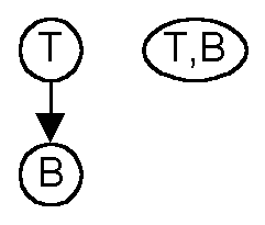
Operations on the Resource Dependency Graph

Consider the figure above. T and B are resources and T depends on B. T continues to run only if B continues to run, so the probabilities that each keep running do not need to be considered separately. For the purpose of the threat calculation we can collapse T and B into one node T,B. The threats against T and B are merged with an adjustment described later.

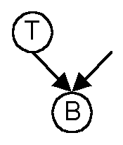
If there were a dependency on B from somewhere else in the subgraph (as in the figure above), the states of B and T must be considered independently. In merging T and B information about the individual states is lost. This information is needed to calculate the probability of failure for whatever is above B and its correlation to T.

If this transformation is applied in a top down manner, there will be no such outside dependency unless there are replica groups. Therefore, an entire resource dependency graph can be collapsed into a single node as shown in the diagram below.

In this diagram C has two incoming dependencies an therefore cannot be merged with either A or B. However, this is not necessary. The transformation is applied in a top down, breadth first manner. Once two nodes are collapsed, the search begins again from the root node. In the first search, A is identified as a viable merger candidate and merged with T. Then the search begins again from T,A. B is identified as a merger candidate and merged to form T,A,B. At this point the dual dependencies converging on C are merged. C is now a merger candidate and is identified on the next pass. It is merged to form T,A,B,C.

Prior to the transformation, the calculation of T's failure probability would have required 4 states. Since each state can be either up or down this results 2⁴ = 16 points in the state space to consider. After the transformation there is only one state and two points in the state space.

Adjusting Threat Descriptions

The threat model models threats against multiple resources, for example power outage or a viral attack. These threats need to be adjusted if their members are merged.

Consider the diagram above. T depends on A and B. A and B are vulnerable to the same threat (the shaded area). When A is merged in to form T,A that threat then applies to B and T,A. There is no problem with this. There is a problem when B is merged to form T,A,B. The probability that the group is attacked remains the same, but the individual probability of failure can change. Consider the case that the threat group is something like vulnerability to the same virus. There is some probability that the system is exposed to the virus, say 0.2. Given that there is viral contamination, there is some probability that either A or B will fail, say 0.1. Merging A and B into T does not change the probability of viral contamination, but the probability T,A,B fails conditioned on the contamination is not 0.1. If the virus infects either A or B, T,A,B will fail. The virus now has two chances against the one node. The correct probability of failure given contamination is P(A or B) = P(A) + P(B) - P(A and B) = 0.1 + 0.1 - 0.01 = 0.19.

Replica Groups

Replica groups impose complexity because their states do need to be considered independently and cannot be collapsed in general. There is some possibility that by exploiting symmetry or approximation this limitation can avoided in common special cases, but we do not have a result in this area yet. Although, we have run down some promising looking box canyons.

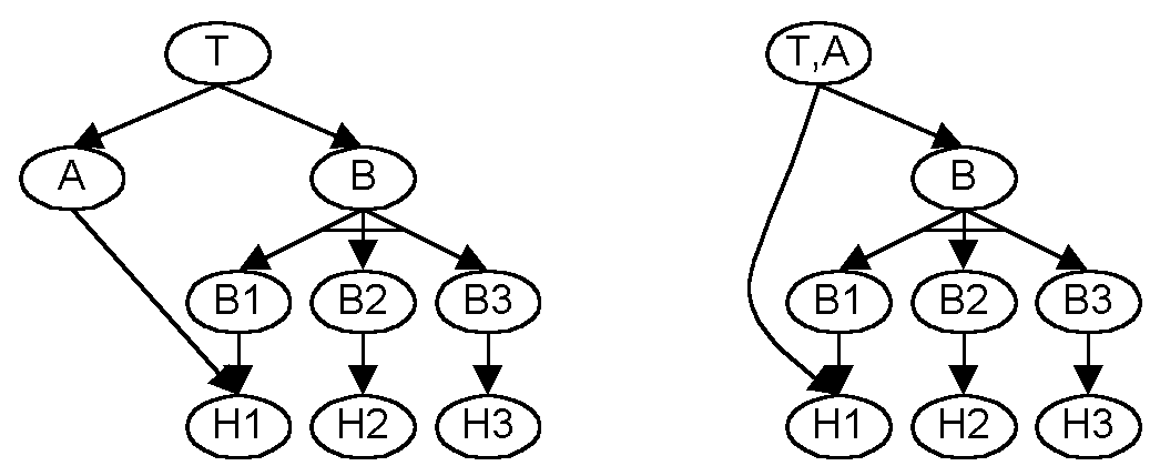
Putting It Together

An example demonstrating a realistic level of complexity is provided.

In the example we have a high level resource T. T depends on a service A which runs on host H1. In addition, T depends on a replica group B. B depends on three replicas B1, B2, and B3. In the diagram the bar across the links indicates an "or" dependency rather than the standard "and" dependency. B1, B2, and B3 depend on H1, H2, and H3 respectively. Applying the transformation once identifies A and merges it to form T,A.

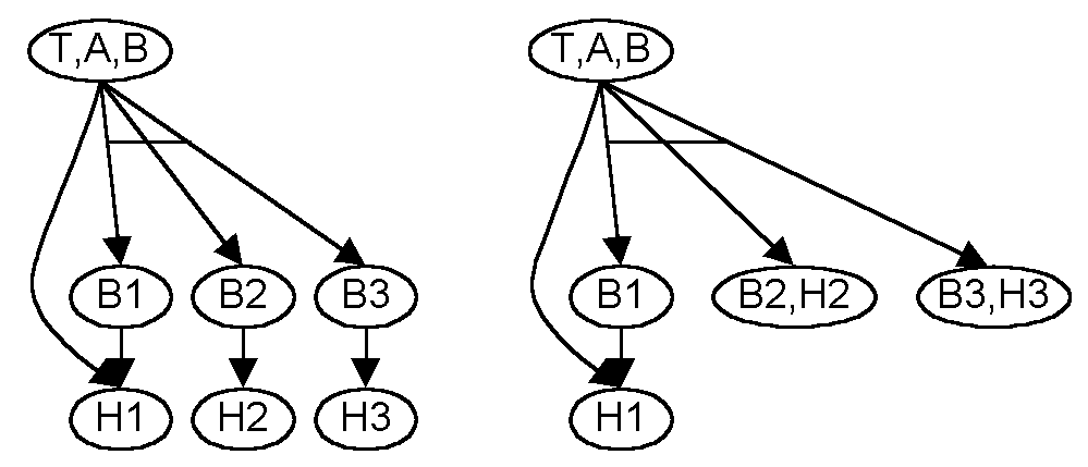
The second application identifies B. Note that in our model we explicitly represent the threat against a coordinator of a replica group as distinct from those of the replicas. B is merged to form T,A,B which has 4 dependencies, A's dependency on H1 and B's dependencies on B1, B2, and B3.

The third and forth applications identify H2 and H3 and merge them into B2 and B3. This is the full degree of compression that we can accomplish with the simple transformation. It has compressed a graph with 9 nodes or 512 points in the state space to 5 with only 32 points in the state space.

5. Issues

5.1. Waste of Resources During Allocation

Self-adaptive systems can waste resources in at least the following ways.

Dedicating the wrong amount of resources to meeting application needs. The obvious example of this would be using too many resources for some purpose. This "over engineering" assigns resources to tasks for which they are not really needed to "make sure" that the task gets done. This is not a problem if resources are plentiful, but can cause other tasks to be starved when resources dwindle. A less obvious example is if the assignment of too few resources to a task causes the task to fail to be accomplished, thereby wasting the resources that were futilely committed.
Excessive optimization. Regardless of the objective function being optimized by the adaptation mechanisms, globally optimal configurations will not be achievable in practice. This means that it will usually appear that a slight "tweaking" of the system could result in a better configuration. However, this is misleading, since the model serving as the basis for optimization contains many errors and uncertainties as outlined above. This uncertainty means that once a certain level of "goodness" has been reached, it will be impossible to tell whether a given adaptation makes the situation better or worse. Bounding the uncertainty tells when further adaptation is pointless.
Optimizing the wrong thing. It will be impossible to make adaptation decisions about all parts of the system simultaneously because it would be very expensive. An understanding of errors can help determine which parts of the system might be furthest from their desired state and thus are most deserving of attention.
Fast vs. ideal decisions. Given the model uncertainty, is it better to make many quick, possibly quite sub-optimal adaptation decisions, or fewer, better decisions more slowly. Since decision quality will be bounded by model uncertainty, should the resources invested in reaching a decision be tunable to tailor the sophistication of the decision making to the model quality?

An understanding of errors and uncertainty (below) is necessary (but not sufficient) to avoid these kinds of mistakes.

5.2. Errors and Uncertainty

The quality of the adaptation decisions that can be made is clearly constrained by the fidelity with which the model reflects the real world. Model infidelities can lead to invalid configurations that do not function properly. They can also cause the decision process to fail to find legitimate adaptations or to perform functionally valid but sub-optimal adaptations. Modeling errors and uncertainty can arise from faulty specifications, sensing errors, errors in assumptions about future behavior, and data management inconsistencies.

To date, little work has been done to determine the effect of modeling and sensing errors on the ability of self-adaptive systems to adapt well. Additional work is needed to understand types and sources of errors and uncertainties that can occur in self-adaptive systems and understand the effect of such errors and uncertainties on the quality of the adaptation decisions that can be reached, and determine ways to ameliorate the effect of such errors and uncertainties.

Errors and uncertainty can creep into a survivable system from several sources (discussed in more detail below):

module and physical resource specifications,
sensed state and events,
assumptions about future behavior,
anomalies due to distributed models and decision making, and

5.2.1. Specification Errors

A survivable system requires specifications of a variety of things in order to be able to construct a robust configuration and correctly recover from failures. Errors in the specifications can cause undesirable behavior. Specification vulnerabilities arise from:

Invalid capability advertisements and requirement specifications. Self-adaptive systems assume that the capabilities of functional modules and the resources they need to provide that functionality can be known to the processes making adaptation decisions. If these are unknown it will be impossible to physically instantiate functional units or connect them to other functionality they need. If the information is incorrect, invalid configurations are likely to result. The obvious way to obtain such information is by developer written specifications that are either stored in a repository somewhere or available by introspection from the components themselves. It is also theoretically possible to generate at least some of these specifications from the design information produced during module development, although this is definitely an open research area. It is not clear how to deal with errors of this type other than to have some sort of feedback mechanism to flag potential errors when they are discovered. For our purposes, we assume that these specifications exist and are accurate.
Incompatible schemata. If the specifications described above come from many sources as will likely be the case in open systems, there is a danger that it will be impossible to accurately match requirements with capabilities. Schema incompatibility is a well known problem that we are not attempting to solve.
Imprecise specifications. The amount of information in capability and requirements specifications needs to be bounded to make their production and management tractable. A danger is that if specifications are not defined in enough level of detail it will be impossible to determine whether matching can be done. An analysis of the appropriate level of detail, while outside our scope, is important.

5.2.2. Sensing Errors

The state of the adapting system is dynamic and must be monitored. Both the normal operations of the system (e.g., current loading) and exceptional events (e.g., failures) must be tracked. There are many ways in which this sensing can be done, but all are subject to error.

Late detection of failures. Failures are generally not detected until after they have occurred, although in some cases symptoms of impending failure may be detected. The time lag between failure and detection may be significant depending on the type of failure and the sophistication of the detectors. Late detection may cause the system to be in a failed state for a significant time before adaptation takes place. If detection delays are significant, the adaptation mechanisms may be forced to construct conservative configurations to reduce the risk that total failure will occur faster than it can be repaired; this will consume additional resources. Estimating a bound on such delays should provide information about how much redundancy is needed to compensate.
Misclassified failures. Failure detectors map observed symptoms of errors to the errors themselves. The more precise this determination can be, the better the adaptation to the failure can be. For example, if it is known that a particular host failed, a reasonable adaptation would be to migrate functionality to an identical host. However, if it were known that the host failed because of a viral attack that was specific to that class of host, such a migration would not be a good adaptation strategy. Mapping symptoms to specific failures is far from a perfect process. Assuming that failures are detected at all, they may be misclassified (e.g., determined to be viral attack when in fact it was a disk sector error) or classified too broadly (e.g., host X failed without giving a reason). It is possible, in principle to trade off between these two kinds of misclassification, accepting broader error determinations in an attempt to ensure that they are correct. It appears useful for the adaptivity decision mechanisms to know the bias of the detectors and classifiers and possibly be able to tune them.
Sampling errors. Performance and loading information probably cannot be continuously sampled, since to do so would pose unacceptable overhead. Instead it is sampled; these samples are of course susceptible to sampling error. The decision process should have insight into the accuracy and timeliness of such samples. This would be useful in the following example. A reasonable strategy when adapting to meet a quality of service goal is to configure in a way that might be sub-optimal, but is less likely to have performance outside the desired range. To do this, it is necessary to bound the probability that performance will fall outside the desired range; this is function of both the variability in the performance of the resource and the uncertainty with which its performance has been measured.

5.2.3. Uncertainty in Assumptions About Future Behavior

When adaptations are performed, it is useful to consider not just the present configuration that will result, but also how that configuration is likely to behave in the future based on some expectation of future events. If a system is adapting to make a particular data source more robust by replicating it, the desirable number of replicas certainly depends on whether they are being placed on Tandem Non-Stop machines or on Windows NT machines.

These estimates of future events are "uncertain" in the sense that it is impossible to objectively determine some truth against which the estimate can be gauged. Examples of the kinds of estimation uncertainty to which this portion of the model is susceptible are:

Uncertainty about threat probabilities. To avoid adapting into a configuration that is either too brittle or that wastes resources, it is useful to know what kinds of things can go wrong and how likely they are. This is termed a threat model and describes both intentional attacks and accidental failures. Some threats are reasonably well understood statistically and can probably be modeled rather accurately; failure rates for hardware are examples of this. Infrequently manifested physical threats such as fires are more problematic; their infrequency makes it hard to accurately quantify their severity. Even worse are intentional attacks whose occurrence is at the whim of an attacker who can (attempt to) mount them at times to be most disruptive; gathering statistics on these will be extremely difficult. For such attacks, it is not even clear that probabilities are the best way to describe their severity or frequency. Even if an appropriate language can be determined, it is not clear how to estimate the severity of a threat that can be imposed or withheld at will.
Failure to correlate failures. Failures and attacks obviously correlate as discussed above. However, because of the difficulty of diagnosing the root causes of failures, it is possible that resource failures that result from the same vulnerability are ascribed to different causes. Conversely, it is possible that independent failures are wrongly ascribed to a common cause. At issue are how to measure or estimate such correlation and the effect of incorrect estimates.
Correlated attacks. It is also possible that the occurrence of certain kinds of attacks may be an indicator that other attacks are impending and should be guarded against by an adaptation. For example, if the number of attacks against particular parts of the system increase, it might be reasonable to assume that other similar parts of the system might be attacked also, or that other kinds of attacks might be mounted against the components already under attack.
Time-varying threat probabilities. The severity of threats can be situational or can change over time. Assuming a static threat model is unreasonable, but mechanisms to evolve the model need to be evaluated. A related issue is how to model and assess attacks that become more likely to succeed over time. Password guessing is a trivial example of such an attack. If it were known how to handle such kinds of attacks it might be possible to "preemptively" adapt the system before it succumbed.

5.2.4. Errors Due to Distributed Models and Decision Making

Errors or inconsistencies can introduced by the distributed nature of self-adaptive, survivable systems. The decision process and model must both be highly distributed. The distributed model cannot be kept synchronous, since such a transactional model of data management would form a choke point. The following kinds of inconsistencies may occur in a distributed environment.

Inconsistencies due to propagation delays. Adaptation decisions will be made with different, possibly conflicting models due to delays in the propagation of sensed information. If model consistency is required for a particular decision, it would be useful to bound how long information takes to propagate.
Inconsistencies due to variable levels of model detail. It is unlikely that all model detail will propagate everywhere, even given arbitrary time. Localization of adaptation decisions and local control of resources (I don't get to use your computer without your permission) will tend to cause local parts of the system to be modeled at greater detail than remote parts of the system. Decisions made based on these differing views may be inconsistent. It would be useful to know in what ways and to develop strategies to have adaptation decisions made using the best available model.
Inconsistent adaptation decisions. Two parts of the system may choose to independently adapt in conflicting ways. This is sometimes called "The Gift of the Magi Problem" in game theory, after the mutually detrimental behavior exhibited in the O. Henry story.

© Copyright 1999 Object Services and Consulting, Inc. Permission is granted to copy this document provided this copyright statement is retained in all copies. Disclaimer: OBJS does not warrant the accuracy or completeness of the information in this document.

This research is sponsored by the Defense Advanced Research Projects Agency and managed by Rome Laboratory under contract F30602-96-C-0330. The views and conclusions contained in this document are those of the authors and should not be interpreted as necessarily representing the official policies, either expressed or implied of the Defense Advanced Research Projects Agency, Rome Laboratory, or the United States Government.

Last updated 5/13/99 sjf

state	after T_destroyed	after T_power	after T_virus
RRRR	0.9900	0.9801	0.96294825
RRRF	-	-	0.00735075
RFRR	-	-	-
RFRF	-	-	-
FRRR	0.0100	0.0099	0.00972675
OTHER	-	0.0100	0.01997425